How to Make a Gantt Chart in Excel: A Step By Step Guide

If you have project deadlines to keep track of, Gantt charts are excellent visual tools. Here is how to make your own on Excel.

Invented by Henry Gantt, Gantt charts are used for project management. They create a visual representation of your project plan to keep track of. You can break down any project into chunks. Setting deadlines is simple so you can follow the project through to completion. Each bar on the chart represents the task duration.

Project managers love this for keeping track of team assignments. But anyone can use one to great effect if you are a solopreneur too. Gantt charts are just perfect charts for projects large or small. This step by step tutorial will show you how to transform a blank Excel sheet into a project schedule.

Here’s What We’ll Cover:

How to Build a Gantt Chart From Scratch 

How to Build a Gantt Chart in Excel Step-by-Step

Key Takeaways

How to Build a Gantt Chart From Scratch 

What are the building blocks of this simple scheduling tool? 

We can summarize as follows: 

• Timeframe
  
  Your horizontal axis should show the intended timeline for the project. This can be broken down into whatever time period you need – weeks, months, or even years
  
  
• List of Tasks
  
  You need to break down your project into several tasks that can be tracked on the Gantt chart. You can also assign each of the project tasks to members of your team.
  
  
• Bars
  
  This is what makes the Gantt chart recognizable. The bars instantly make it stand out as they show the progress of your project. Visual scheduling helps monitor progression.
  
  
• Dateline
  
  A dateline is a vertical indicator of the present date. You will be able to look at your visual schedule and instantly see where you are up to.
  
  
• Goals and milestones
  
  You could also call these deadlines. What are the key dates that certain items need to be delivered to the client?
  
  

How to Build a Gantt Chart in Excel Step-by-Step

There is free Gantt chart creation software on the internet, but many people like to use Excel. This is where the power of Excel really comes to play.

Follow this simple guide and you can customize your own project management tracker. 

Step 1. Label the first three columns, “Task”, “Start” and “End”.

We recommend putting the labels in A4, B4 and C4 to leave room at the top.

Step 2. Input your task list. Enter the task start dates and task end dates into the column.

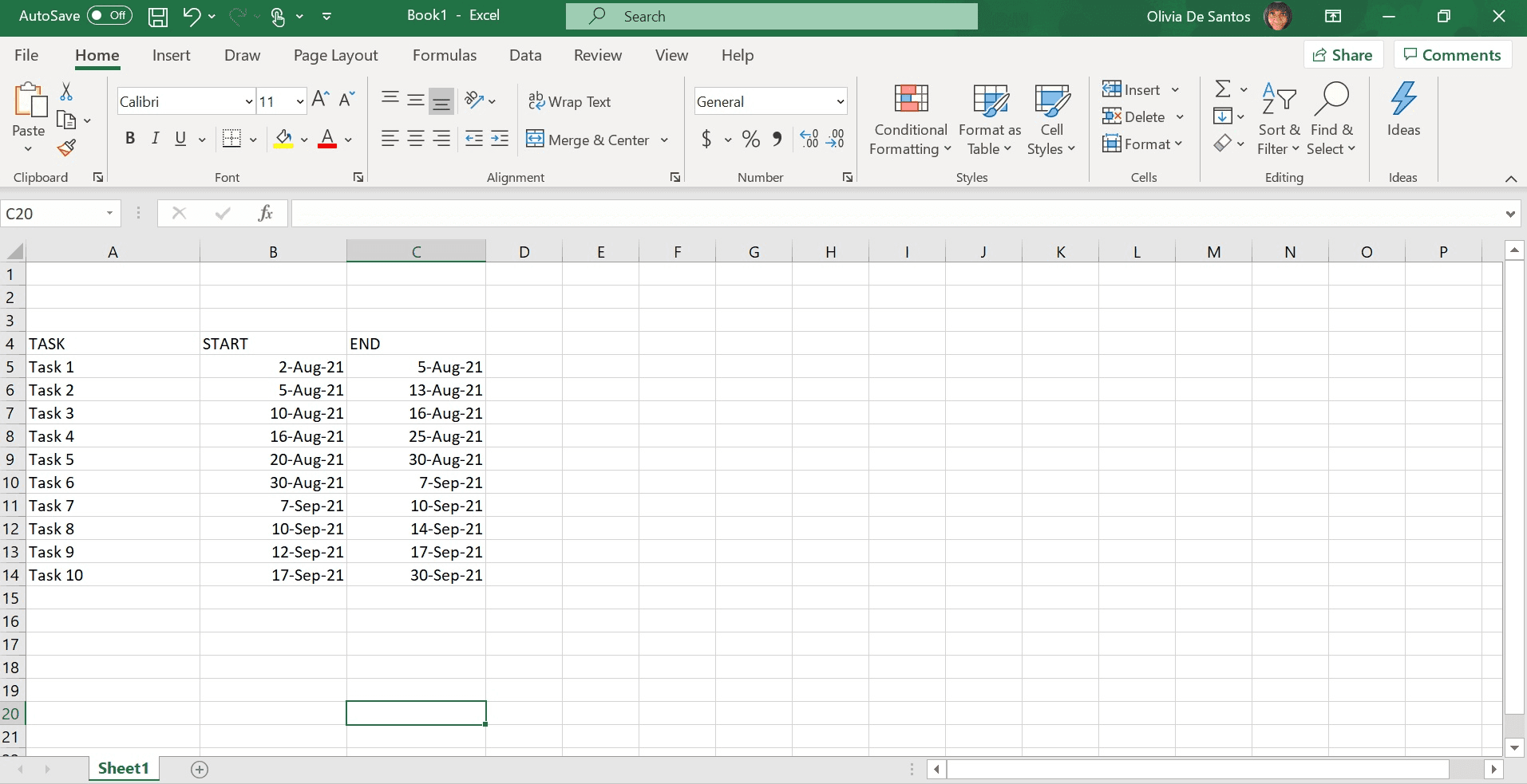
Make sure the dates are in the default date format.

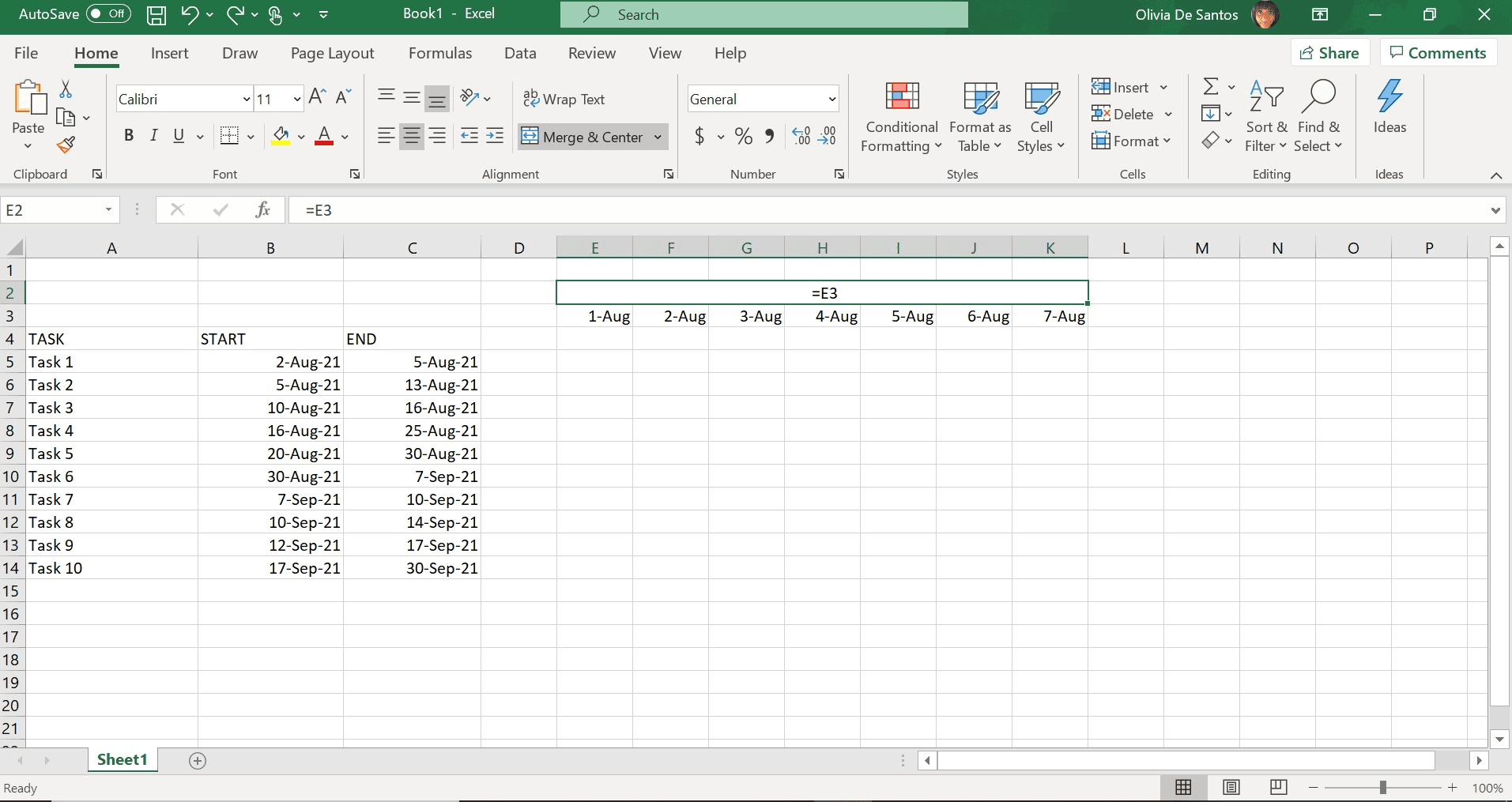
Step 3. Now time to create the date range for the project timeline. 

I did this with the first 7 dates for now starting with the 1st of the month for ease.

Step 4. Merge the cells above the line of 7 dates you have entered. Make the merged cell equal to the first date.

In my case, the formula was =E3

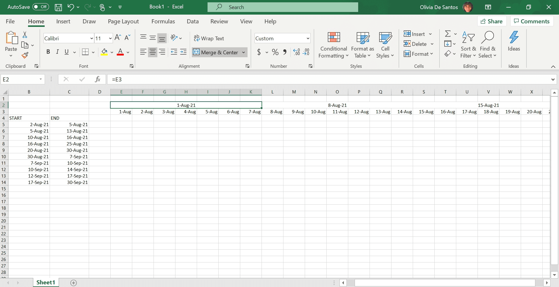
Step 5. Select the group of 7 columns and copy them to the right.

Step 6. Enter the project start date in the top left

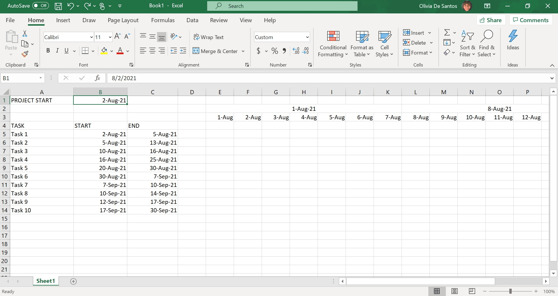
Step 7. Connect the start date to the first date in the chart.

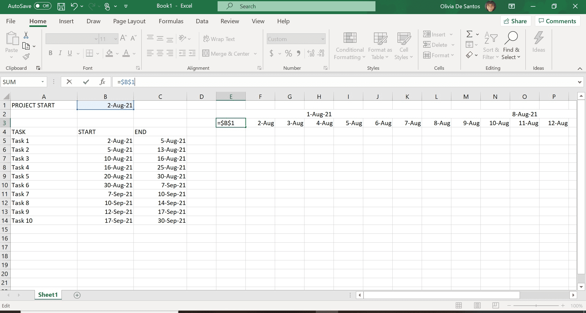
To do that, select the first date in your project timeline. In my case this was the 1st of August. 

I delete the contents and input the formula =B1

Then I click FN4 and the formula will automatically change to =$B$1

Click the enter bar and the date will change.

Step 8. Now we need to make sure that the following dates follow a sequence. 

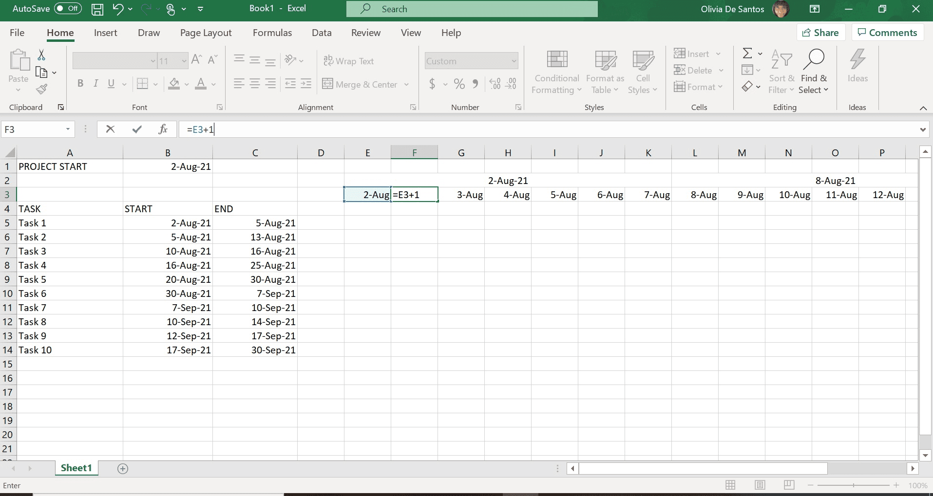
Select the next date in the timeline and put in = the previous cell + 1

For me that was =E3+1 

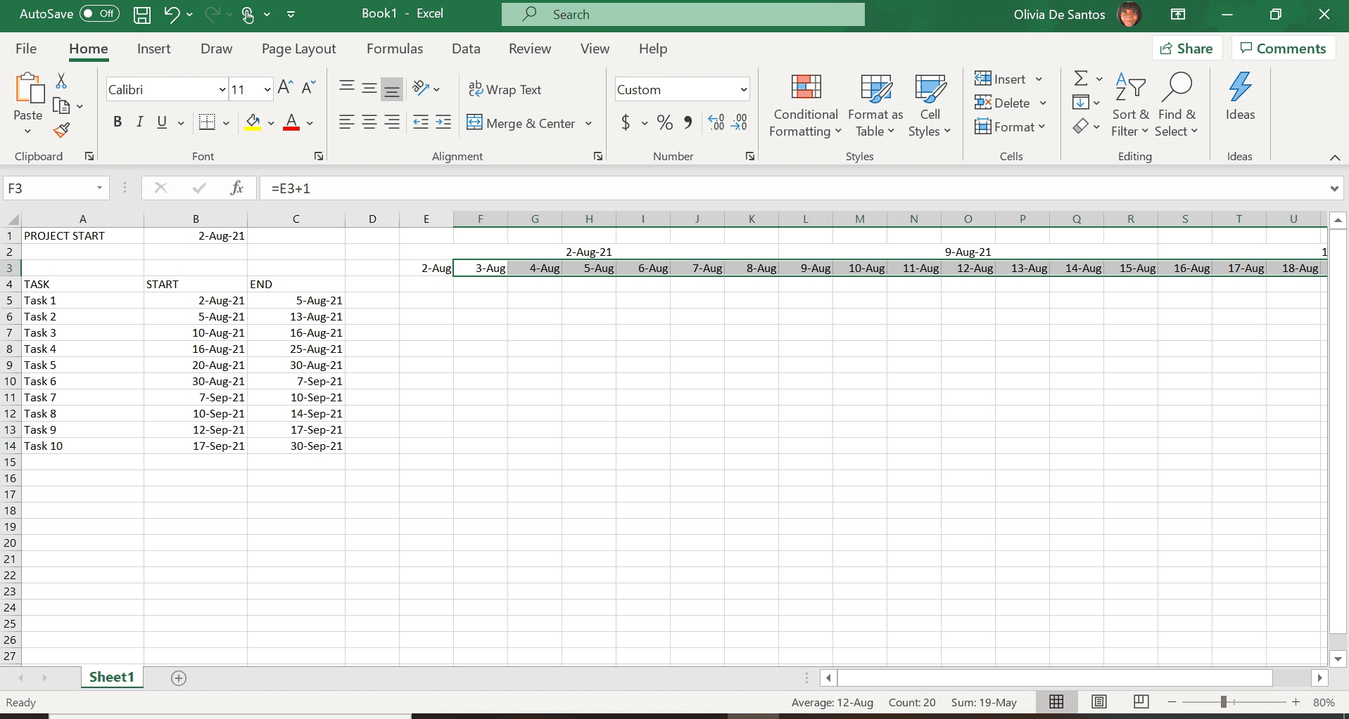
Use your cursor to drag the formula across the entire row. 

Now whenever you change the project start date in the top left corner, the entire project timeline will automatically change. (How cool is that?) 

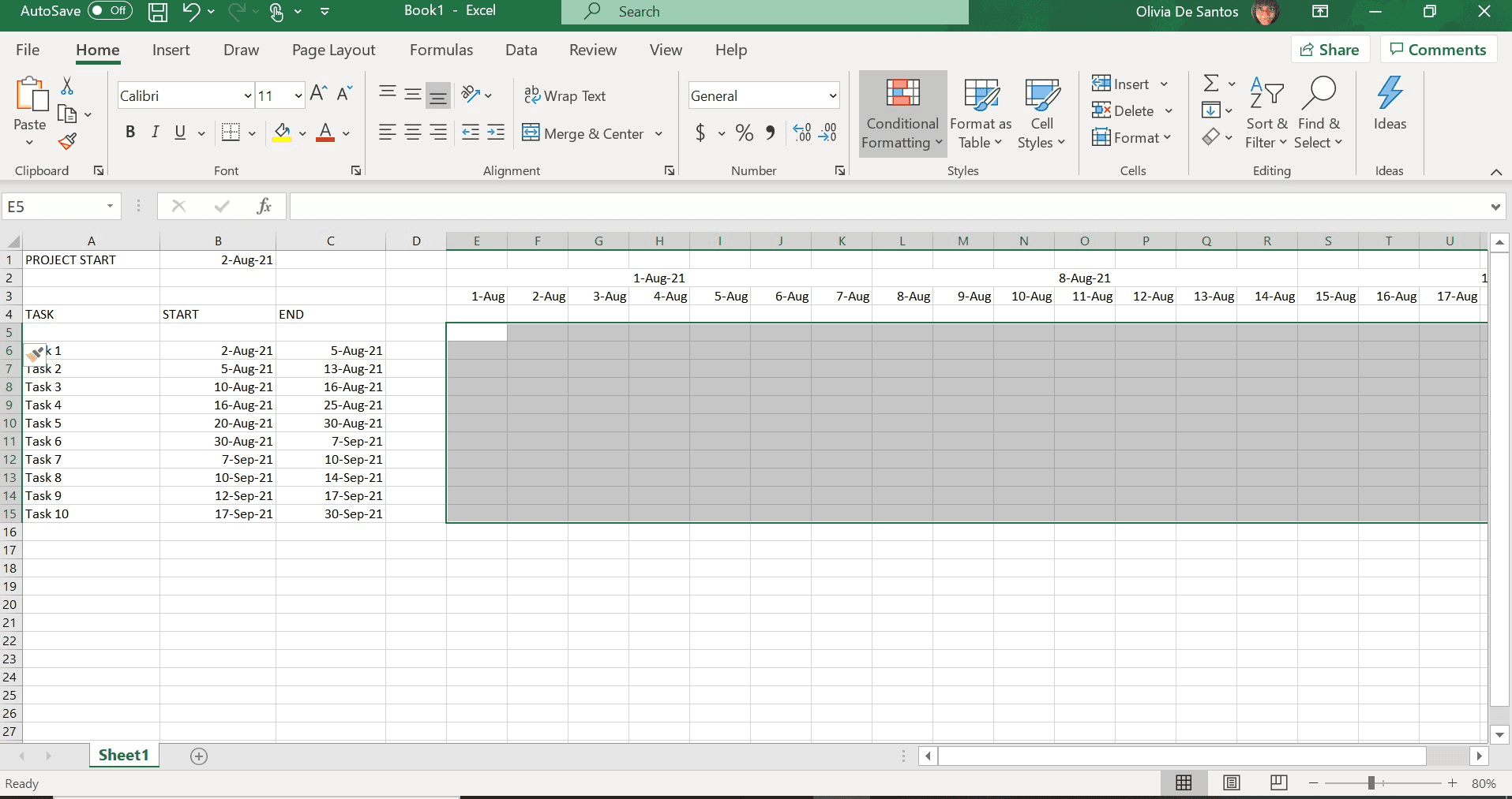
Step 9. Now to make the bar chart. We want to create conditional formatting so that an automatic bar chart is created at the project’s start date and end date. 

Proper formatting is what makes the taskbars dynamic and automatic.

Use the selection tool to select all of the cells that align with the project timeline. 

Then select “conditional formatting” on the format tab of the header menu.

Step 10. Select “new rule” on the drop-down menu of conditional formatting rules.

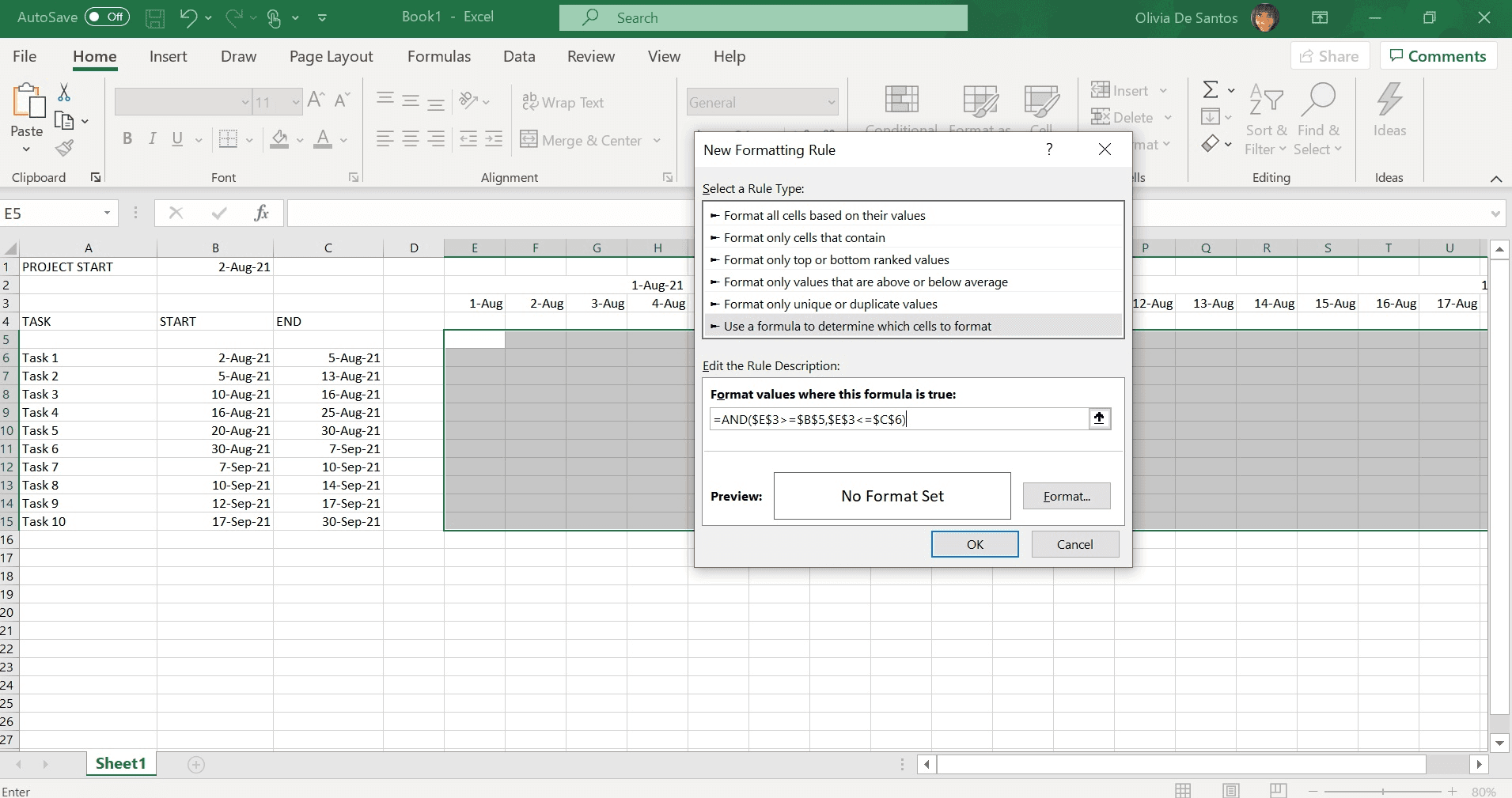
 Step 11. Select “use a formula to determine which cells to format. 

Step 12. Start entering your formula as follows

=AND([select top left cell of your project timeline] >= [space under START], [select top left cell of your project timeline] 

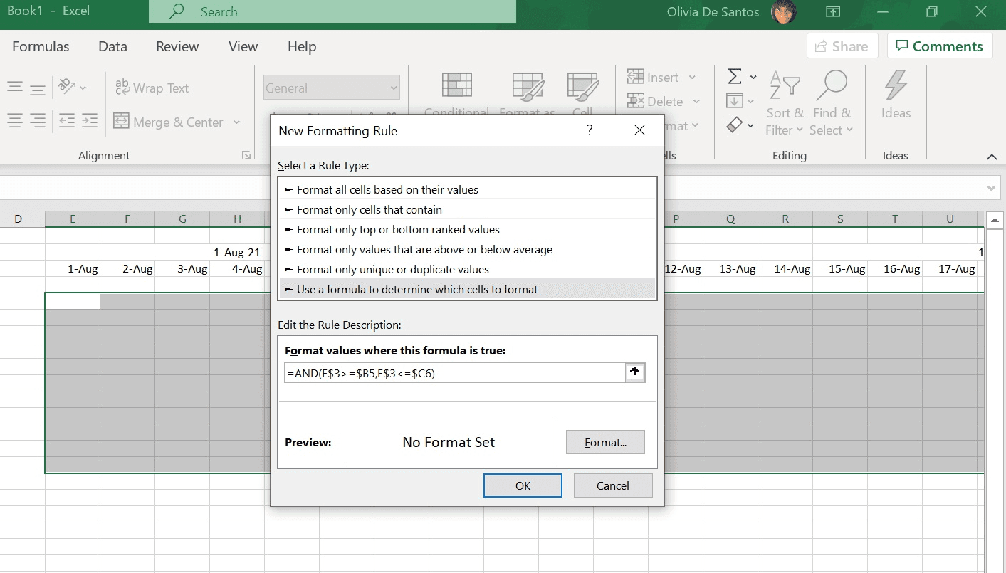
Step 13. Now take out some of the dollar signs from the formula so it looks like the image below. 

Step 14. Select “format” > fill. Choose a color from the color tab.

The fill color you choose will show up as your bar colors. If you don’t choose a color or pattern, you will accidentally make the bars invisible!

Step 15. Congratulations! You have made a simple Gantt chart with Excel! 

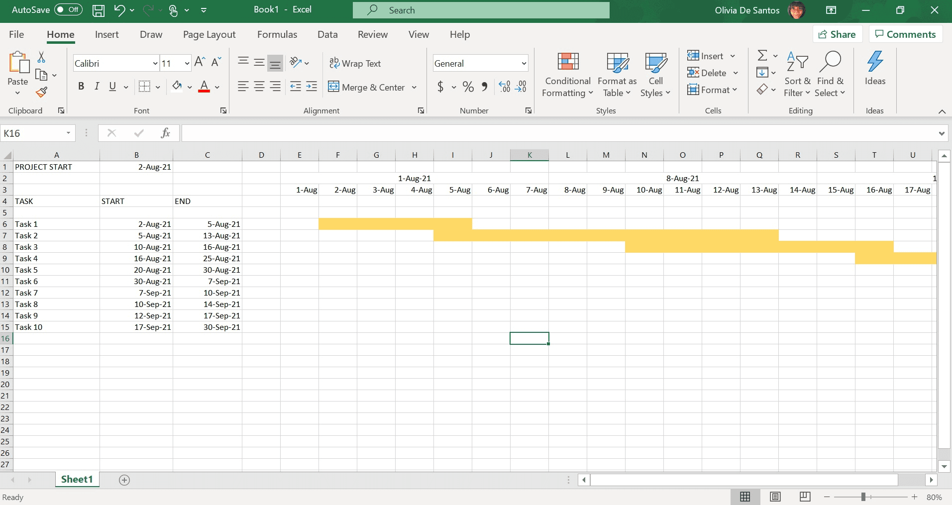
You can use any additional formatting you choose to make your Gantt chart more legible.

Key Takeaways

We hope this Gantt chart guide helped you create a usable productivity chart for your team. If Excel is a bit complicated for you, don’t worry. You are not alone! There are plenty of Gantt chart templates on the internet. A pre-built Gantt chart template can save you time and effort.

For more Excel and productivity guides like this, head to our resource hub!

---

RELATED ARTICLES